Acquiring correction images for the shading correction
Switching shading correction on or off
Defining the magnification range
Having a look at correction images for the shading correction
See also
Acquiring correction images for the shading correction
Prerequisites:
•The microscope should be thoroughly aligned.
•The beam intensity should be stable.
•If you are using the Tengra or Quemesa cameras, a camera calibration has to be carried out. The camera calibration is carried out only once before the camera is used for the first time.
Carry out the following steps to acquire correction images for the shading correction.
|
|
|
|
|
|
|

Preparing the microscope
Make typical settings for your work on the transmission electron microscope.
1.Set the acceleration voltage that you usually work with.
2.Set a magnification between 12000 x and 20000 x to make the illumination as homogenous as possible. If your microscope can be controlled via remote control by your software, there are two alternative ways to set the magnification.
•You can set the magnification on the microscope itself. Then the magnification you've set will automatically be transferred to your software and displayed in the Microscope Control tool window.
•You can also enter the magnification in the Microscope Control tool window. The transmission electron microscope's magnification will then be correspondingly adjusted by remote control.
3.Make sure that the fluorescent screen is evenly lit. The electron beam should be widened so that the whole fluorescent screen is evenly illuminated. Widen the beam until it is at least 10% bigger than the fluorescent screen.
4.During the acquisition of the shading correction images, no sample should be in the light path. With some microscopes, you can put the sample into a parking position. Alternatively, you can find a hole of sufficient size in your sample.
When you are working with a microscope without remote control
Check whether the high voltage and the magnifications are already defined in the Device Settings dialog box. If necessary, define the magnifications and the high voltage that your microscope has or the ranges with which you work. As a rule, you only have to specify these fundamental settings once.
Prerequisite: In the Device List dialog box, you have selected the TEM Without Remote entry from the Microscope picklist.
1.Open the Device Settings dialog box with the Acquire > Devices > Device Settings... command.
2.Select the Microscope > Column > General entry in the tree view.
3.Set the high voltage that you are working with.
4.Select the Microscope > Column > Magnification entry in the tree view.
5.Enter the magnification in the Define magnifications field.
6.Click the Add button to add the magnification to the List of magnifications list.
7.If necessary, add further magnifications which you use.
8.Confirm your settings with OK.
9.Set the magnification on the microscope in which you want to create correction images for the shading correction.
10.Make sure that your software displays the same magnification in the Microscope Control tool window.
11.Make sure that the fluorescent screen is evenly lit. The electron beam should be widened so that the whole fluorescent screen is evenly illuminated. Widen the beam until it is at least 10% bigger than the fluorescent screen.
12.During the acquisition of the shading correction images, no sample should be in the light path. With some microscopes, you can put the sample into a parking position. Alternatively, you can find a hole of sufficient size in your sample.
Preparing image acquisition
If you don't have shading correction images and you click the Live button, you get an error message. Switch shading correction off temporarily to be able to create a live-image. You will find step-by-step instructions for doing this further below
1.Switch your software to the Acquisition layout. To do so, select the View > Layout > Acquisition command.
•In this layout, all tool windows that you need for the image acquisition are automatically displayed.
2.Click the Live  button in the Camera Control tool window on the left edge of the user interface.
3.If the microscope can be controlled by remote, the beam blanker is automatically deactivated.
4.If your camera is mounted on the side of the transmission electron microscope, the camera will automatically be moved into the column.
If your camera is mounted below the microscope column, the fluorescent screen will be raised.
5.If the Manual observation method was active, this observation method will automatically be deactivated.
6.The Auto Contrast option in the Adjust Display tool window is automatically switched on in order to display the image optimally.
3.Make sure that the Automatic option in the Exposure group of the Camera Control tool window is selected.
•In the image window, you see the live-image. If no shading correction images have been acquired yet, you will see shading artifacts in the image.
•The live image's intensity distribution is displayed at the top of the Adjust Display tool window. All 14-bit cameras have an intensity value range between 0 and 16,383.
4.Set the intensity of the electron beam on the TEM so that the displayed exposure time is between 500ms and 2s. Make sure that the image area remains evenly lit.
5.Click the Live  button again, and exit the live mode.
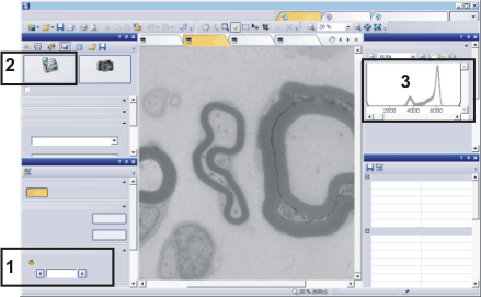
Your software's user interface in the Acquisition layout looks like this. You will find the tool windows that you need for the image acquisition here. Set the microscope magnification in the Microscope Control tool window (1). Switch to the live-image in the Camera Control tool window. (2). You can see the live image's intensity distribution at the top of the Adjust Display tool window (3).
Starting calibration process
The process flow for the actual acquisition of correction images will be controlled by a wizard. This wizard will guide you through the procedure step by step. Then follow the instructions given you by the software wizard. It takes several minutes to acquire all the correction images. The correction images will be saved automatically.
There are several ways of starting the software wizard:
1.To do so, you can use the Acquire > Calibrations... command. Select the Shading Correction calibration process in the Calibrations dialog box and click the Calibrate... button.
2.In the toolbar of the Camera Control tool window, click the Acquisition Settings  button. Select the Camera > Adjustment entry in the tree view. Click the Calibrate... button in the Correction group.
3.You can find more information on the calibration process' process flow here.
Testing shading correction
1.Click the Live button in the Camera Control tool window on the left edge of the user interface. Have a look at the live-image. The shading artifacts should have disappeared.
•You can use the Line Profile tool window to check the shading correction. Remove the sample or move to a hole in the sample. Measure the intensity diagonally across the whole image. The line profile should now be a straight line.
You can find more information on the Line Profile tool window here.
2.Check whether the shading artifacts are also being corrected in other magnifications.
•If shading artifacts are still appearing in certain other magnification ranges, you should acquire a correction image for these magnification ranges. You will find step-by-step instructions for doing this further below
3.Click the Live button again, and exit the live mode.
Switching shading correction on or off
Using shading correction, your software can remove image structures that originate in the imaging system and don't belong to the actual image information.
Switching on the shading correction
1.Make the Camera Control tool window appear. To do this, you can use the View > Tool Windows > Camera Control command.
2.In the Camera Control tool window, click the Acquisition Settings button in the tool window's toolbar.
3.The Acquisition Settings dialog box opens.
3.Select the Camera > Adjustment entry in the tree view.
4.In the Adjustment dialog box, select the Flatfield entry from the Shading list to activate the flatfield correction. With the flatfield correction, you will automatically also activate the dark current correction.
It is also possible to switch on the dark current correction only. Select the Dark current entry from the Shading list.
5.You will find an explanation of the terms flatfield correction and dark current correction here.
5.If you have not yet acquired correction images, acquire correction images now. You can find step-by-step instructions on how to acquire the correction images above.
6.Confirm the settings with OK.
Switching off the shading correction
1.In the Camera Control tool window, click the Acquisition Settings button in the tool window's toolbar.
2.Select the Camera > Adjustment entry in the tree view.
3.In the Adjustment dialog box, select the Off entry from the Shading list.
4.Confirm the settings with OK.
Defining the magnification range
In a transmission electron microscope, the imaging conditions change significantly in different magnification ranges. For example, different lenses are used to realize a lower magnification. Or the image is rotated significantly when you switch into a different magnification range.
For example, define three magnification ranges with low, medium and high magnifications. Acquire your own correction images for the flatfield correction for each magnification range.
Note: If you change the magnification ranges, all current flatfield correction images will be deleted.
1.Use the Acquire > Calibrations... command.
2.Choose the Shading Correction entry in the Calibrations list.
3.Click the Edit... button.
•The Edit Shading Images dialog box opens. Here, you find a list of entries showing all the correction images that have been acquired. The magnification range for the correction images is also shown.
Defining the magnification range
4.In the Edit Shading Images dialog box, click the Edit Magnification Ranges... button.
•The Edit Magnification Ranges dialog box opens. All magnification ranges that have been defined are listed here. A magnification range is predefined by default which includes various magnifications that your transmission electron microscope offers.
5.Set up a new magnification range. To do so, select the magnification that represents the upper limit of the new magnification range in the Magnifications list. You can click the Add button to specify a new magnification range.
•In the Upper range limit list, a new magnification range has been specified. The upper limit of the magnification range is the magnification you selected. The lower limit is automatically set so that all the possible magnifications of your transmission electron microscope are assigned to precisely one range.
6.Move the mouse pointer over an entry in the Upper range limit list to look at the lower and upper limits of the selected magnification range.
7.Close the Edit Magnification Ranges dialog box with OK.
•A dialog box appears warning you that all flatfield correction images will be deleted.
8.Confirm whether you want to have the current flatfield correction images deleted.
9.In the Edit Shading Images dialog box, only the dark current correction images are still listed.
Acquiring new flatfield correction images
1.Close all dialog boxes.
2.On the microscope, set a magnification that is in the lowest magnification range.
3.Start the Shading Correction calibration process. You don't need to acquire the dark current correction images again. Acquire the flatfield correction images for the current magnification range.
•For each magnification range, exactly one set of flatfield correction images is acquired. One set of flatfield correction images is composed of exactly one correction image for each possible camera resolution.
4.On the microscope, set a magnification that is in a different magnification range. Acquire the flatfield correction images for the current magnification range.
5.Open the Edit Shading Images dialog box.
6.In the Edit Shading Images dialog box, you'll now find a set of flatfield correction images for each magnification range. Each set contains flatfield correction images for all available camera resolutions.
6.Close the dialog box with OK.
Having a look at correction images for the shading correction
All correction images that are acquired in the Shading Correction calibration process are saved automatically. You can look at this images at any time. Use this option, for example, when the shading correction isn't working properly. Correction images that weren't acquired properly could be the cause of this.
1.Open the Edit Shading Images dialog box.
•To do so, use the Acquire > Calibrations... command. Choose the Shading Correction entry in the Calibrations list. Click the Edit... button.
2.In the dialog box's list, choose the correction image that you want to view.
3.Click the View button.
•The selected correction image will be loaded in the document group.
•By default, the correction image's name is composed of all the information that is specified in the Edit Shading Images dialog box: <Shading Type>+<High Voltage>+<Magnification Range>+<Resolution>.
4.You can now save the correction image just as you can every other image.
00284 28112014